

PPC marketers spend a lot of time in spreadsheets analyzing data and creating various reports. Often this is done using PPC formulas in Microsoft Excel.
When Google Sheets first launched in 2006, while being free, it was very basic and lacked a lot of the functionality that Microsoft Excel had. However, Google has continued to improve Google Sheets to a point where it now has some really cool functionality that PPC experts can benefit from.
For basic PPC formulas on Excel, be sure to read my blog 13 Microsoft Excel formulas for PPC marketers. While Microsoft Excel is very powerful and has its benefits, there are a handful of formulas and functions in Google Sheets that make it very useful for PPC marketers.
In this article, I will be discussing my favourite 12 PPC formulas for Google Sheets that are not available in Excel.
12 PPC Formulas You Need To Know


1. FILTER
Use FILTER to quickly find search terms that meet your criteria
If you have your raw search query data stored in Google Sheets, you can use the FILTER formula to create several tables that are useful to you. This makes it a lot easier to find searches that you need to act on.
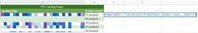
The first part of the filter formula selects the data that will be retrieved. The next part is the criteria that needs to be matched. For example, if you want to see all search terms that have spent more than £75 and have zero conversions, then you would use the below formula:
=FILTER(Range, Criteria Range, Criteria, Criteria Range 2, Criteria 2) 
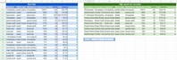
You can use the idea above to create a dashboard of different tables that will help with your search query analysis. Here are some examples of the kind of tables that you could create and why you may find them useful:
- Search terms that have spent more than a certain amount of money and have not converted – consider adding these as negative keywords
- Search terms that have converted more than three times and came through a non-exact match keyword – Consider adding these in as exact match keywords
- Search terms that have a good number of impressions but have a low CTR – Take a look at the ad copy to see if CTR can be improved or maybe it is isn’t a relevant search term and needs to be blocked out
- Search terms that have a decent amount of volume, a very high conversion rate and came through a non-exact match keyword – Add as an exact match keyword and give it a high bid
2. IMPORTRANGE
Pull data from other sheets with IMPORTRANGE
Sometimes you need to access some data that already exists in another sheet. If you don’t want to do the work again, then you can use the IMPORTRANGE formula to pull the date from the other sheet automatically. To do this, all the formula needs is the URL of the other sheet, the name of the tab that the data is stored in and the cell range to retrieve.
Bear in mind that certain types of formatting, like the background colour, font size or font style, will not make its way into the new sheet.
=IMPORTRANGE("Google Sheet URL","Tab name!Range")
3. IMPORTXML & IMPORTHTML
Scrape data on the website with IMPORTXML or IMPORTHTML
The IMPORTXML and IMPORTHTML formulas are extremely powerful and can be used to help with a variety of problems. These formulas can be used to scrape various parts of a web page
There is a bit of a learning curve when it comes to using the IMPORTHTML and IMPORTXML formulas which is out of the scope of this blog. However, here is a basic example of how you could scrape the data from a website to help with PPC marketing
One such example of using the IMPORTXML formula is to keep an eye on the number of products on a page. Clothing websites often have products going in and out of stock regularly. Usually, pages with a low variety of products will have a poor conversion rate because there just aren’t enough variety of products on the page. The good news is that with the IMPORTXML function, you can monitor the number of products on the page and then pause the landing page that doesn’t have a lot of products. This means that you can divert the budget to other pages that have more products and are likely to have a better conversion rate.
To monitor the number of products on the page, you need to have a look for something on the page that mentions the number of products on the page and then pull that into Google Sheets.

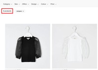
We need to look into the source code of the landing page to see the text that we need is stored. This does take a bit of knowledge in HTML and also some knowledge in how to use the IMPORTXML formula.
However, in our case, the number of products text is stored in a div class that is called ‘ProductCount__product-count___3sehe’. So, all we need to do is tell the formula to retrieve whatever is stored in the div class that is called ‘ProductCount__product-count___3sehe’.

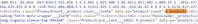
We can do this with the below formula. Once we have the basic formula, we can add in all of our PPC landing pages in one column and then add the IMPORTXML formula in another column to monitor the number of products on that page.
=IMPORTXML(CELL,"//div[@class='ProductCount__product count___3sehe']")
4. IMAGE
Add an image using a URL
If you’re creating a report in Google Sheets, adding an image can help to make a point or to make your spreadsheet look more professional. There are other ways to add an image, but one way is to use the IMAGE function. This will add an image into the cell that the formula is added in. You can make the image larger and smaller by increasing the size of the cell.
=IMAGE(“URL”)

5. GOOGLETRANSLATE
Translate any ad copy to English
If you’re running PPC advertising in another language and need to get an idea of what your ad copy or keywords mean, you can use the GOOGLETRANSLATE function.
The GOOGLETRANSLATE function has three parts, and each part is split up by a comma. The first part requires the text to be translated; the second part requires the language that the text is in, and the last part is the language that the text is to be translated to.
=GOOGLETRANSLATE(CELL,"de","en")

If you’re not sure what is the code of the language that the text is written in, then you can use the DETECTLANGUAGE function.

6. UNIQUE
Deduplicate rows of text quicky
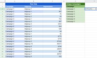
Microsoft Excel has an option where you can easily remove duplicates, but Google Sheets doesn’t have a solution like this unless you add an Extension. One solution is to use the ‘UNIQUE’ formula to remove any duplicates. For example, if you need to remove all duplicated campaigns so that you only have unique campaigns, then you could use the below formula:
=UNIQUE(Range)
7. QUERY
Create a ‘top ten’ table
Using the Query function in Google Sheets, you can show the top 5 or top 10 highest figures within some raw data. You can use this formula to surface the top five keywords with the highest impressions or the top ten converting keywords, for example. You can read a more detailed blog on how to do this here.
=QUERY(RANGE, “SELECT Column Names Order by Column Name Desc Limit 10”)
8. GOOGLEFINANCE
Convert currency
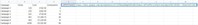
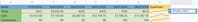
Google Sheets can use Google’s currency conversion capabilities directly within Google Sheets. You can do this with the GOOGLEFINANCE formula. This is especially useful if you do international PPC and need to convert the data into your currency.
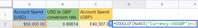
To perform the currency conversion in Google Sheets from USD to GBP, you can use the below formula. In the below formula, ‘USD’ is the current currency and ‘GBP’ is the new currency. This formula will give you the currency conversion rate. You then need to Multiple the old currency with the currency conversion rate to get the value in the new currency.
=GOOGLEFINANCE("Currency:USDGBP")
9. SPARKLINE
Basic graphs for reporting purposes with sparklines
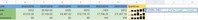
It is easy to add a small graph that will give an idea of the direction the data in your report is going with SPARKLINES. These are perfect if you want to provide a visual representation of the data, but a full graph is not required. You can create Sparklines in Microsoft Excel, but would say that the method of doing so is a lot simpler in Google Sheets.
=SPARKLINE(Range)
You can also change the chart type from a line graph to a bar graph. There’s a lot more that can be done with SPARKLINES but these two
=SPARKLINE(Range,{"charttype","column"})
10. QUERY
Find what metric of a keyword needs to improve to increase its Quality Score
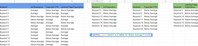
The Quality Score of your keywords are broken down into three metrics: Ad relevance, Expected Clickthrough rate and Landing Page Experience. So, to start improving the Quality Score of your keywords, you first need to know where each keyword is lacking. To quickly see this information, you can insert your Quality Score data into Google Sheets and then use the QUERY function to show all keywords that score a ‘Below Average’ for any of the relevant Quality Score metrics.
To create the QUERY function, the first part tells the range that it should look in. The next part tells Google Sheets what data to retrieve and the criteria to look for. You can do this for each of the three Quality Score metrics.
=QUERY(RANGE,"SELECT A,B WHERE B='Below Average'",FALSE) 
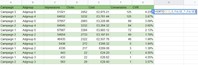
11. SORT
Surface the most valuable data in a range to the top with SORT()
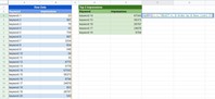
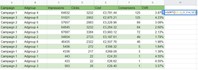
You can use the SORT function to sort your raw data so that the most valuable data appears at the top. For example, you may want to see the highest spending ad groups or the highest converting ad groups at the top.
The SORT function requires the range where the raw data can be found and then the number of the column to sort with. So, for example, if you want to sort with the sixth column in your range, then you would add six over here. Lastly, you would add TRUE if you want it to sort from ascending order and FALSE if you want it to sort from descending order.
Another popular option is to create a filter and then sort for whatever criteria you want. However, the benefit of using the SORT function is that if you refresh your raw data, your sort data will automatically refresh itself. Here is an example if you want to sort by having the highest converting ad groups at the top.
=SORT(RANGE,6, FALSE)
We can also sort by multiple criteria. In the below example, the SORT function will show the highest converting ad groups at the top. However, where it finds ad groups with the same number of conversions, it will show the ad group with the highest CVR first.
=SORT(RANGE,ROW NUMBER, TRUE/FALSE)
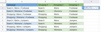
12. SPLIT
Easily split text within campaign names with Split()
In my campaign naming convention, I like to have a pipe that separates key information. This is because I can then use formulas to group data in specific ways and improve my data analysis capabilities.
Unfortunately, Google Sheets does not have a ‘Text to Columns’ option like Microsoft Excel does that allows you to segment campaign name data into separate rows. In this case, you can use the SPLIT function to segment essential parts of the campaign name into different rows.
I always separate important parts of my campaign names with a pipe, but you can use whatever you’re comfortable with. To create the SPLIT function, the first part includes the cell that the function should look at. The second part is the criteria that it should look when deciding where to split the campaign name text.
=SPLIT(CELL,” | “)
Wrapping Up
So there are my 12 Google Sheets formula tips for PPC experts. There may be other ways to achieve the same thing in Microsoft Excel, but the actual formulas are not available in Microsoft Excel.
I’ve tried to give example use cases for each formula, but once you’re comfortable with using these formulas, there is a lot more than you can do with them.
In many instances, the above formulas can be combined to enable you to carry out much more complex data analysis. While doing your day to PPC work, start having a think about how you could use the above formulas to do complete work faster or better.


